R Tutorial in Logistic Regression

Recently I read a paper that used logistic regression in its methods and realized I had no idea what logistic regression is, so I made this tutorial for myself and others to learn about it. I wanted to create a tutorial that created random data that anyone could use, and taught you a bit about R in the process. This is my first tutorial and feedback is encouraged.

This tutorial on the statistical machine-learning method known as Logistic Regression is implemented in R. Familiarity with programming syntax, such as vector indexing, is assumed but I tried to make this tutorial as accessible as possible for those with less programming experience.

What in Merlin’s beard is logistic regression?

First, what is regression?

You may have heard of “linear regression,” which fits a $y=mx+b$ line to a set of points, such as in the figure below. I’m not going to go into the details of linear regression, but you can read about it if you like.

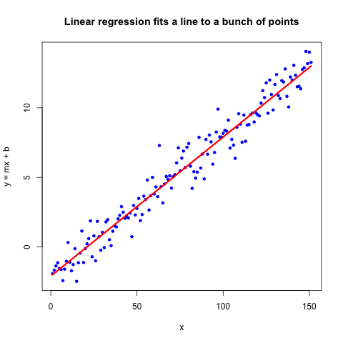
Logistic regression is similar, but instead of having two continuous variables as above, one of the variables is binary (0 or 1) and the other is continuous. But we’re not fitting a line, we’re fitting a logit, which is a totally different function that estimates probability for a continuous variable rather than assigns classification. For example, we could predict the probability of cancer relapse given some gene expression values. Or the probability of a heart attack given a person’s cholesterol levels. We would base these probabilities on previously encountered data, a method of machine learning known as “Supervised Learning.” You tell the computer what the answer is for many examples, and then the computer has to guess whether the outcome is 0 or 1.

Think of it this way: you look at hundreds of values representing the number of Star Trek: The Next Generation episodes a person has watched, with a teacher peering over your shoulder, and he tells you whether each value is associated with attending a Star Trek convention or not. Then the teacher leaves, and you’re given a new number of Star Trek: TNG episodes, $x$, and you have to give a probability $p$ whether the person who has seen this many episodes has been to a convention. The probability of $x$ episodes watched and no convention attendance is $1-p$, so by knowing $p$, we also know $1-p$ and we only need to specify one value.

Regression is not the same thing as classification

This is an important distinction between classification and regression. If we were doing classification, we would just say whether the person who has seen $x$ number of episodes has gone to a convention or not. But we don’t always want a binary outcome. The cholesterol-heart attack association is a great example of this. You probably don’t want to tell a patient, “You will have a heart attack,” but rather say “You have an $x$% probability of having a heart attack, given your current cholesterol levels.” Same goes for cancer relapse. A binary yes/no answer can obscure the data. Also, a probability of 0 is essentially impossible. Could you truly, definitively, say that a person will never have a heart attack? Not until their death, but then all possible heart attack events have already been observed. Sorry for the gruesome-ness.

So what about this logisitic thing?

First, we have to talk about odds

We talked about predicting the probability of some event. But we’re going to use odds instead. If the probability of having attended a Star Trek: TNG convention is $p$, then the odds are:

$$\text{odds} = \frac{\text{probability of event ocurring}}{\text{probability of event not occuring}} = \frac{p}{1-p}$$

Say after watching a certain number of episodes, the probability of attending a convention is $p=0.7$. Then the odds of attending a convention are

$$\frac{0.7}{0.3} = 2.333\ldots$$

But the odds of not attending a convention are

$$\frac{0.3}{0.7} = 0.4285\ldots$$

As you can see, odds and probability are not the same. Odds can be greater than 1, and probability must be between 0 and 1.

Next, we have to define log-odds

It would be nice if these odds were somehow symmetric and we could intuitively make inferences just by looking at the value. This is where the logarithm comes in. If we take the natural log (ln), aka $\log_e$ of the odds of attending a convention, we get

$$\ln \frac{0.7}{0.3} = 0.8472\ldots$$

And the log-odds of not attending a convention:

$$\frac{0.3}{0.7} = -0.8472\ldots$$

The opposite of attending a convention is the negative of attending a convention! Now let’s stop and think. Why is this? This is because the natural log of 1 is 0, so it intersects at 0 as in the plot below. Then the natural log of anything smaller than 1 is negative, approaching negative infinity as the number gets closer and closer to 0. The natural log of anything larger than 1 is positive, and approaches positive infinity as the number gets larger and larger, but slower than we approach negative infinity from the other side.

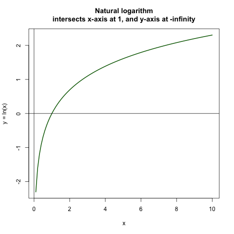
This symmetry is helpful to guide our intuition about events occurring or not occuring.

FYI: We used the natural logarithm here because that’s the standard. You could really use any log base you like, even $\log_\pi$ would do, but it’s just not used that often.

From log-odds to logits

The log-odds are also called the logit of the probability:

$$ \log(\text{odds}) = \text{logit}(p) = \ln\left( \frac{p}{1-p} \right) $$

In logistic regression, we set

$$\text{logit}(p) = a_0 + a_1x_1 + a_2x_2, \ldots , a_nx_n$$.

Where $n$ is the number of independent variables you have. In our case, we just have one independent variable, $x = x_1$, the number of Star Trek: TNG episodes viewed. But we could add to the complexity and also have $x_2$ be the number of Star Trek: The Original Series (happy 46th anniversary!) episodes viewed, $x_3$ be number of latinum strips owned, and $x_4$ be Klingon language proficiency. But we’re going to keep it simple and stick to our one $x$.

Now we could do regular ol’ linear regression on this, but there are several issues.

1. We have a binary variable for our dependent variable (aka the $y$), and linear regression assumes a continuous distribution for the dependent variable. With probability as the output, we cannot have values less than 0 or greater than 1, and linear regression does not conform to this.
2. The variance of $y$ is not constant across values of $x$. The variance is $p(1-p) = pq$ ($q$ is short for $1-p$), and if we have a probability of $0.50$ of attending a Star Trek convention, then we have $0.5\times 0.5 = 0.25$ odds. But if we have $p=0.9$, then the variance $pq = 0.9\times 0.1 = 0.09$, and $0.25 \neq 0.09$. Thus the assumption that variance of $y$ is constant across values of $x$ is invalid. This is also called homoscedasticity.
3. If you want to do significance testing (you maybe familiar with p-values or R-values to describe how significant a result is), the assumption that the errors of prediction, $Y-Y^\prime$ are normally distributed doesn’t work. $Y$ only takes on the values 0 and 1, so there’s no way you can create a continuous distribution such as a normal distribution with just two values.

Logits are not very intuitive as a unit, even though they are very helpful when looking at odds. But we need to get back to probabilities so we can give a probability of convention attendance. We’ll have to exponentiate both sides to get rid of the natural log. I’m going to keep the long-form version of the equation so you can see how it works for more variables.

$$ \begin{align} \text{logit}(p) &= \ln\left( \frac{p}{1-p} \right) = a_0 + a_1x_1 + a_2x_2, \ldots , a_nx_n\newline \frac{p}{1-p} &= e^{a_0 + a_1x_1 + a_2x_2, \ldots , a_nx_n} \newline p &= (1-p)e^{a_0 + a_1x_1 + a_2x_2, \ldots , a_nx_n} \newline p + p(e^{-(a_0 + a_1x_1 + a_2x_2, \ldots , a_nx_n)}) &= 1 \newline 1 + e^{`(a_0 + a_1x_1 + a_2x_2, \ldots , a_nx_n)} &= \frac{1}{p}\newline \frac{1}{1+e^{-(a_0 + a_1x_1 + a_2x_2, \ldots , a_nx_n)}} &= p \end{align} $$

We can multiply the fraction by a clever form of 1, $e^{(a_0 + a_1x_1 + a_2x_2, \ldots , a_nx_n)}/e^{(a_0 + a_1x_1 + a_2x_2, \ldots , a_nx_n)}$ to get

$$ p = \frac{e^{(a_0 + a_1x_1 + a_2x_2, \ldots , a_nx_n)}}{1+e^{(a_0 + a_1x_1 + a_2x_2, \ldots , a_nx_n)}}. $$

If we set $a_1 = 1$ and all other $a_0, a_2, a_3, \ldots = 0$, then we get the general logit cuve below

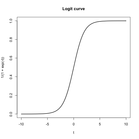
So now we have a way of creating a predictor of the probability of a binary variable from a continuous variable. Now let’s get started with doing regression.

PS, if you want to get math typesetting (aka LaTeX) on your blog, I recommend against searching for “tumblr latex” and instead checking out this tutorial on installing MathJax on your blog, tumblr or not.

Step 1: Get binary data.

Initialize a vector of 0’s

For this case, we are going to make up some binary data. According to a nice explanation of logistic regression, logistic regression requires at least 50 data points per classification. Meaning, 50+ 0’s and 50+ 1’s. There are 178 total Star Trek: TNG episodes and lots of bonus features and interviews on the DVDs, so let’s round up to 200 total TNG pieces of video. In R, rep is the function to create a vector of repeated values. The first argument is what you want repeated, and the second argument is how many times you want to repeat it. You could even have a vector in the first argument, such as rep(c("red", "blue"), 30), to get a vector of alternating strings, “red” and “blue.” We could have also made the same vector with classification = vector(length=200, mode="numeric"), which initializes the numeric values at 0, but I decided to do it with rep instead.

classification = rep(0,200)

EDIT: I’ve been informed that at 50+ data points is not always necessary, so take the rule with a grain of salt.

Set a random seed

Let’s set the random seed so we will get consistently the same results, no matter how many times we run the code. No random number generator is truly random, and part of the semi-randomness is starting with a seed number, and then doing all kinds of transformations to then get a “random” number. So if we make sure we are always using the same seed, then we will always get the same set of “random” numbers.

set.seed(100)

Randomly add 1s to the last part of the vector

Now let’s randomly add a bunch of 1s to the vector, ramping up the probability of getting a one (with hyperbolic growth, if you’re being technical) as we get to the end of the vector. Let’s be interesting and add some noise to the data so we don’t have not do an equal 50/50 split. We’ll use a randomly-generated probability distribution to assign 0 or 1 to the last 125 values. This way, our data is a little more realistic and less clean.

FYI, runif is the uniform distribution function in R, which has an equal probability of obtaining every value between 0 and 1. It is useful in this assignment because I know that the odds are 50/50 that the value will be greater than 0.5, so I increased the threshold to >0.6 and added a multiplicative factor, which varies from 1 to 125. This way, the values near the beginning of the vector have close to a 60/40 chance of being less than 0.6, but by the end, they are almost certainly all above 0.6. Take a look below.

The multiplicative factor: FYI, the str function is a method of previewing the first few values of variables without seeing everything at once. It can be handy. Another method is head, which like the *NIX head, shows the first few values, but it can be annoying if you have a matrix with a large number of columns, say over 100. Then you get the first 10 values for all 100 columns, which takes up a lot of space. str can be more convenient in that case.

> str(125/125:1)
 num [1:125] 1 1.01 1.02 1.02 1.03 ...

Randomly generated values in the uniform distribution: (Notice that I re-set the random number seed. This is because after a random seed is used, the random number generator advances to the next seed.)

> set.seed(100); str(runif(125))
 num [1:125] 0.3078 0.2577 0.5523 0.0564 0.4685 ...

Multiplicative factor times the uniform distribution vector: (For those Linear Algebra lovers out there, we don’t get a matrix because by default, R multiplies vectors on an element-by-element basis. If you want the usual vector product, aka the cross product, do vector1 %*% vector2)

> set.seed(100); str(runif(125)*(125/125:1))
 num [1:125] 0.3078 0.2598 0.5613 0.0578 0.484 ...

Now we can use ifelse to assign a 0 or 1 based on whether the vector we just created is greater than 0.6 or not.

set.seed(100); classification[76:200] = ifelse(runif(125)*(125/125:1) > 0.6, 1, 0)

The final binary vector

This is what I get for the binary classification vector. Keep in mind that we only added 1’s to the last 125 values, or from index 76 and up.

> classification
  [1] 0 0 0 0 0 0 0 0 0 0 0 0 0 0 0 0 0 0 0 0 0 0 0 0 0 0 0 0 0 0 0 0 0 0 0 0 0
 [38] 0 0 0 0 0 0 0 0 0 0 0 0 0 0 0 0 0 0 0 0 0 0 0 0 0 0 0 0 0 0 0 0 0 0 0 0 0
 [75] 0 0 0 0 0 0 0 1 0 0 0 1 1 0 0 1 1 0 0 0 1 1 1 1 1 0 0 1 1 1 0 1 1 0 1 1 1
[112] 0 1 1 0 0 1 1 1 1 1 1 1 0 0 0 0 0 0 1 0 0 0 1 0 1 1 1 1 1 1 1 1 0 1 1 1 1
[149] 1 1 1 1 1 1 0 1 1 1 1 0 1 1 1 1 1 1 1 1 1 1 1 1 0 0 1 1 1 0 1 1 1 1 1 0 1
[186] 1 1 1 1 1 0 1 1 1 1 1 1 1 1 1

Step 2: Get some continuous data.

We’re going to make up continuous data similarly to how we created the binary classification vector. This time, we set the next seed so we’d get different numbers, and multiplied a uniform distribution by a linear function. Now this isn’t quite enough to make most of the 1’s be in the upper numbers and most of the 0’s be in the lower numbers, so we add a linearly increasing amount of Gaussian noise to the values.

set.seed(101); continuous = runif(200)*1:200+rnorm(200,mean=50,sd=5)*1:200

My continuous vector looks like this:

> str(continuous)
 num [1:200] 51.7 94.2 184.1 226.1 269.9 ...

As you can see, we have values larger than 200, but we assumed there are 200 pieces of Star Trek: TNG video media to watch, so we need to normalize it by the max. Now our maximum value is 1, so we multiply by 200 to get a maximum value of 200.

> continuous = continuous/max(continuous) * 200

What does our data look like?

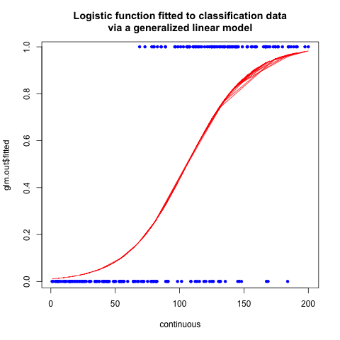
Now if we plot the continuous vector vs the binary vector, we’ll see that in general, the 0’s occur in the lower end of the continuous spectrum, and the 1’s occur in the higher end of the continuous spectrum.

png("~/workspace/tutorials/logistic_regression_points.png")
plot(continuous, classification, pch=20, col="blue")
dev.off()

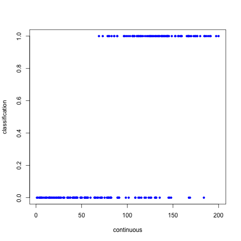
So according to our data, there’s a lot of people who have seen most of Star Trek:TNG and have been to a convention, but there are a few individuals who have seen most of it and yet have not been a convention.

Step 3: Do logistic regression!

Now you can use generalized linear models to fit to the data. Note: This is one of many methods in R to do logistic regression, and I chose to do the simplest version. Note that classification ~ continuous is shorthand for y ~ x, or as the R people say, response ~ terms. If you had more data points, like Klingon language profiency, you would add this variable by using the cbind or “column bind” function which would create a 2-column matrix from the two vectors: glm(classification ~ cbind(continuous, klingon), ...).

glm.out = glm(classification ~ continuous, family=binomial(logit))
png("~/workspace/tutorials/logistic_fitted.png")
plot(continuous, glm.out$fitted, type="l", col="red", lwd=1, main="Logistic function fitted to classification data\nvia a generalized linear model")
points(continuous, classification, col="blue", pch=20)
dev.off()

The plot of the fitted curve looks like:

So what actually happened here?

The glm function found the values of $a_0$ and $a_1$ that minimize the error term. I’m not qualified to describe glm in gory detail, or all the other possible methods of calculating logistic regression, but this site gives the mathematics the justice it deserves. You will need to be familiar with linear algebra to fully understand the arguments.

FAQ

What if your classification is 1 for the low values and 0 for the high values?

You can still use the same steps, but your logit curve will be flipped along the $y$-axis.

Have you attended a Star Trek convention?

No, I have not. But I thought it would be a fun binary variable.

References

I could not have done this without the help of many different sources.

• http://luna.cas.usf.edu/~mbrannic/files/regression/Logistic.html - the first thing I read, and the primary source for the explanation of logistic regression in the first section (What in Merlin’s beard is logistic regression?). Highly recommended introduction to logistic regression.
• http://en.wikipedia.org/wiki/Logistic_regression - Wikipedia is a great place to start, but it dove into the technical aspects a little too quickly for my taste.
• http://www.statgun.com/tutorials/logistic-regression.html - a great explanation of logistic regression in general.
• http://ww2.coastal.edu/kingw/statistics/R-tutorials/logistic.html - used R to explain logistic regression of a particular dataset.
• http://www.omidrouhani.com/research/logisticregression/html/logisticregression.htm - mathematical derivation of logistic regression
• http://ww2.coastal.edu/kingw/statistics/R-tutorials/logistic.html - explains logistic regression and odds, and implements logistic regression on a particular dataset.