May 1, 2014 rna splicing alternative splicing python pandas rna science
If you’ve been reading my blog for general python/productivity stuff, you are in for a TREAT! Here is some REAL SCIENCE! I’ll give a quick intro but please let me know if anything is unclear. I spend most of my time talking to a few people who study this stuff in painful detail, so I’d love to know where my explanation becomes cloudy.
tl;dr: I wrote a small tool for quantifying alternative junction usage from RNA-STAR alignment output: https://github.com/olgabot/sj2psi And it’s on PyPI so you can pip install sj2psi as well.
Alternative splicing is a method of creating different versions of a gene using the same DNA. It is awesome because it increases the possible number of genes in say the human genome from just 30,000 to millions. An extreme example is the Drosoephila (fruit fly) gene Dscam, which has over 60,000 potential versions, more than the genes in the Drosophila genome! Alternative splicing happens by combining different “exons” together (always in linear order) to create different proteins (or other gene products like ncRNAs but we won’t go into that)
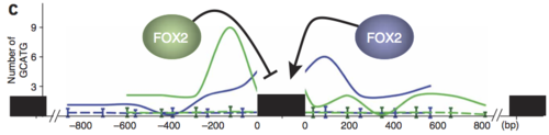
These different versions of the same gene are called “isoforms.” What we care about is looking at individual events because we study RNA binding proteins (RBPs), some of which have an effect on alternative splicing when they bind RNA. So maybe we know that an RBP binds some gene’s RNA, but it (most likely) only has an effect on the exon(s) immediately before or after. For example, the RBP FOX2 is one of our lab’s favorites, partly because our boss found that if FOX2 binds upstream (“before” in DNA terms) of an exon, it suppresses inclusion of it. HOWEVER! FOX2 binding downstream (“after”) an exon promotes inclusion! Check out this figure from Yeo et al, Nat Struct Mol Bio (2009):
Quantifying alternative exon usage and changes is always a challenge, and this is especially difficult for unannotated splicing events. Which is why I was excited when I read a single-cell paper learned of bam2ssj (Paper: Pervouchine et al, Bioinformatics (2013) and its successor, sjcount. The promise is that instead of quantifying whole splicing events which have to fall into some specific category (SE/MXE/RI/A5SS/A3SS/AFE/ALE/TandemUTR, see this figure from Wang ET et al, Nature (2008). Each “box” is an exon and the lines in between exons are stretches of DNA that are removed (called “introns” because they “interrupt” the exons)

Plus these events have to be annotated for use with my splicing quantifier of choice (MISO), or you could try to pull them out from the aligned file. However, I work with single-cell data and since splicing is mostly binary in single cells (i.e. you have mostly isoform A and not both isoform A and B, citation: Shalek et al, Nature (2013)), it becomes a pain to make these annotations, because you have to merge ALL the files together to create like a terrabyte-sized alignment file (usually a *.bam file) and then you are introducing all kinds of craziness because what could have been noise in a few cells gets added up together and becomes signal.
Sigh.
So I’d much rather use something that quantifies splicing of all junctions, arbitrarily. But when I tried using sjcount I couldn’t figure out what one of the outputs was (like what’s the difference between a “splice junction” and a “splice boundary?”). Plus I realized that the “splice junction counts” (*.ssj) file was really similar to the “SJ.out.tab” file created by the RNA-STAR aligner.
.ssj files look like (I added the column names):
chrom   start   stop    strand  overhang    count
chr1    146509  155767  .       20      1
chr1    146509  155767  .       34      1
chr1    146509  155767  .       49      3
chr1    168165  169049  .       10      2
chr1    168165  169049  .       49      3
chr1    694503  700103  .       29      1
chr1    694503  700103  .       41      1
chr1    694503  700103  .       49      1
chr1    894461  894595  .       7       2
chr1    894461  894595  .       9       5
“overhang” is the number of base pairs of the sequencing read that overlaps with the upstream exon of the splicing event. The rest of the read is on the downstream exon. In our case, our reads are 100 base pairs (“100bp”) so if there’s 20bp overhanging on one exon, the other 80bp are on the other exon.
While SJ.out.tab files are (again I added column names):
| \n | chrom | \nfirst_bp_intron | \nlast_bp_intron | \nstrand | \nintron_motif | \nannotated | \nunique_junction_reads | \nmultimap_junction_reads | \nmax_overhang | \n
|---|---|---|---|---|---|---|---|---|---|
| 0 | \nchr1 | \n135332 | \n138297 | \n1 | \nGC/AG | \nFalse | \n0 | \n1 | \n38 | \n
| 1 | \nchr1 | \n146510 | \n155766 | \n2 | \nCT/AC | \nTrue | \n5 | \n1 | \n34 | \n
| 2 | \nchr1 | \n156895 | \n158300 | \n1 | \nGC/AG | \nFalse | \n0 | \n2 | \n17 | \n
| 3 | \nchr1 | \n168166 | \n169048 | \n2 | \nCT/AC | \nTrue | \n5 | \n3 | \n46 | \n
| 4 | \nchr1 | \n169265 | \n172556 | \n2 | \nCT/AC | \nTrue | \n0 | \n2 | \n13 | \n
The start/stop are off by one here because .ssj’s index is from the exon end/exon start, and this is from the intron start/intron end. So the SJ.out.tab coordinates are (start from .ssj+1) and (end from .ssj-1).
FYI, the .ssc files looked like:
chr1    894595  894595  .       8       1
chr1    1228468 1228468 .       1       1
chr1    1228468 1228468 .       3       3
chr1    1228468 1228468 .       5       1
chr1    1228468 1228468 .       6       1
chr1    1228468 1228468 .       7       2
chr1    1228468 1228468 .       12      1
chr1    1228468 1228468 .       13      2
chr1    1228468 1228468 .       16      2
chr1    1228468 1228468 .       27      1
This claims to have the same columns as .ssj files except instead of start/stop it’s position/position. I was very confused by how you can have a count at a position. Why does chr1:894595 have one line while chr1:1228468 have a bunch? If you search for 894595 in the .ssj file, you get:
chr1    894461  894595  .       7       2
chr1    894461  894595  .       9       5
chr1    894461  894595  .       10      2
chr1    894461  894595  .       11      1
chr1    894461  894595  .       12      1
chr1    894461  894595  .       14      1
chr1    894461  894595  .       16      2
chr1    894461  894595  .       19      1
chr1    894461  894595  .       20      1
chr1    894461  894595  .       21      13
chr1    894461  894595  .       22      1
chr1    894461  894595  .       42      2
chr1    894461  894595  .       49      14
How did all these counts in the last column (which sum to 46 by my calculation) become 1 in the .ssc file? I was pretty lost.
ANYWAYS all of this is a buildup to say that I used Pervouchine et al’s method of quantifying alternative junctions as asking, when this upstream exon (splicing donor, D in figure below) is used with this downstream exon (splicing acceptor, A in figure below), how often does that happen relative to all other donors and acceptors? In the figure below, the splicing event of interest is a thick, bold line, joined by a solid arc representing the spliced read. The dotted lines represent that this donor could be spliced to a bunch of different acceptor sites.

This is quantified with a $\Psi_5$ (“Percent spliced-in”, or “Psi” of the donor, which is at the 5’ end of the RNA) and $\Psi_3$ (“Psi” of the acceptor, located at the 3’ end of the RNA) scores:

Where the summation is over all other possible acceptors (in the case of A’) or all other possible donors (in the case of D’).
So using the SJ.out.tab files from RNA-STAR and the magic of pandas, and a bit of filtering, you can calculate these scores very easily:
sj['psi5'] = sj.groupby(['chrom',
    'first_bp_intron'])['total_filtered_reads'].transform(lambda x: x/x.sum())
While this does $\Psi$ scores from raw counts which is frequentist and I prefer to be Bayesian, this is a reasonable start.
Check out the package I wrote for this: https://github.com/olgabot/sj2psi I’d love your feedback and contribution. It’s also available on PyPI, so you can pip install sj2psi and start using it today! It’s under the MIT license so just attribute me :)